how to make negative numbers red in excel

Red-0 and 2 click Apply. Select a red number under Negative numbers then click OK.

How To Make Negative Numbers Red In Excel

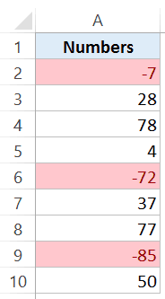
When you are working with lots of different numbers in Excel you sometimes want your numbers to stand out by showing them in a negative red number enclosed in parenthesis.

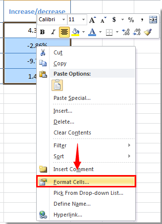
. This is a brief tutorial video demonstrating how to make any negative numbers or percentages that appear in a list red. You will need to app. Select the list contains negative numbers then right click to load menu. It should in the bracket and in red color.

Please see the steps below for details. How to Make Negative Numbers Red in Excel Google Sheets. On Format Cells under Number tab click Number in Category list then in Negative numbers list select number with brackets. Alternatively press Ctrl 1 on the keyboard.

This option will display your negative number in red. Click Format Cells on menu. If your data contains numbers formatted as different types for example both percentages and currencies make sure the cells you highlight contain numbers. Note that Excel allows you to apply special formatting for different types of numerical data such as percentages and currency values.

Microsoft Excel How to Make Negative Numbers Red. In the Format Cells window select RED color under Negative Numbers section. In the Custom number formats window 1 enter the same format used in the Excel example above 0. Under Formatting style 3 click on the Text Color icon and 4 choose.

You will need to app. Before showing you how lets take a moment to demonstrate how to format an individual cell or a group of selected cells to display a negative number in red or with a minus sign. Select the cell or range with numbers. Step2 Then press Enter key and drag the fill handle across to the range that you want to contain this formula.

1Select the range of cells where you want to make negative numbers red and in the Menu go to Format Conditional formatting2. Automatically Format Negative Numbers Red in ExcelBy default negative numbers are not shown in a different colour by default in Excel. Select the range of cells where you want to make negative numbers red and in the Menu go to Format Number More Formats Custom number format. Then click OK to confirm update.

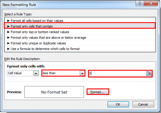
Right-click on the cell and select Format Cells. Select the range you want to change. In the window on the right side of the sheet 1 choose Less than in Format rules and 2 enter 0 in the input box. In Excel you can turn negative numbers to red or add parentheses to make them much easier to read.

Our guide continues below with another way to format negative numbers as red including pictures of those steps. In Excel to solve this task the Conditional Formatting also can do you a favor please do as this. It seems to work based on the first cell so if the first cell is negative all numbers go red and if the first number is positive all numbers go black. In a blank cell says the Cell E1 input the formula IF A1.

Highlight the cells containing your data. In the present case we have given formatting to a negative number as Red ie. You can create a custom format to quickly format all negative percentage in red in Excel. In Excel the basic way to format negative numbers is to use the Accounting number format.

Then click OK to confirm update. Right-click on a selected cell. With the target cells highlighted click on Format Cells or right-click Format Cells. Open your Excel file.

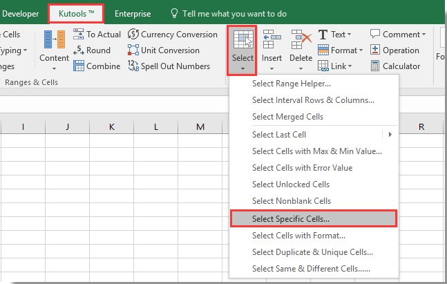
Hi all Im trying to write code that allows me to make negative numbers red and positive numbers black for a highlighted range of cells. Now we want to make all negative numbers in red. Click Kutools Content Change Sign of Values see screenshot. Select the cells to change.

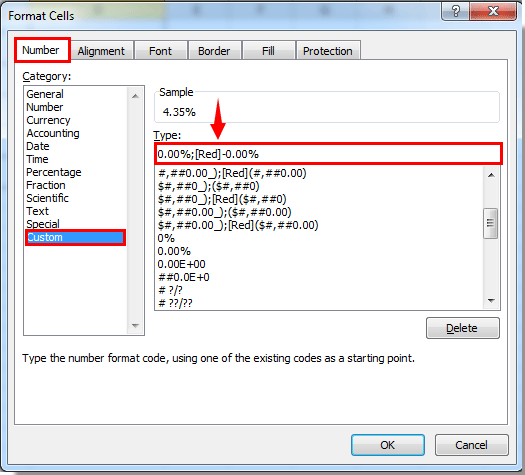
Select the list contains negative numbers then right click to load menu. Mark negative percentage in red by creating a custom format. Select the cells which have the negative percentage you want to mark in red. On Format Cells under Number tab click Custom then under Type enter 0Red-0.

Format the cell value red if negative and green if positive with Conditional Formatting function. Verify that after above setting all. On the Number tab select the category Number and change the format to the second or fourth option negative numbers have red color and the - sign is shown. Click OK at the bottom.

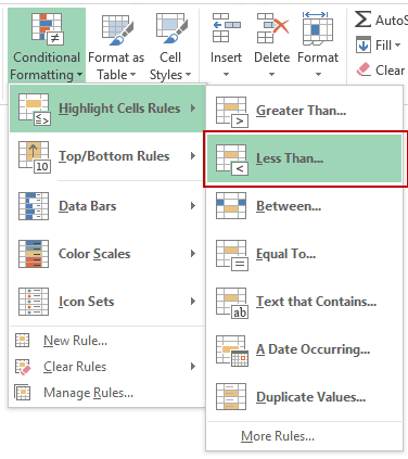
If you have installed Kutools for Excel you can change positive numbers to negative as follows. Select the numbers that you want to use and then click Home Conditional Formatting. But for some reports negative numbers must be displayed with parenthesis. How to Make Negative Numbers Red in Excel 1.

The third part denotes the formatting of zero 0 in the cell The fourth and the last section denotes the formatting of the text Characterswords. The Microsoft Excels IF function can recognize negative numbers and change them to zero without affect positive numbers. Click Format Cells on menu. Make All Negative Numbers Red by Format Cells Setting.

Click Number under Category. To do this you need to select your numbers and press CTRL1 to bring up the Format dialogue box. Right click to bring up the dialog box from the list click Format Cells.

How To Make All Negative Numbers In Red In Excel